[분류모델] 02. Decision Tree
Decision Tree (의사결정나무) : 변수들로 기준을 만들어 샘플을 분류하고 분류된 집단의 성질로 추정하는 모형
종속변수의 종류가 범주형이면 분류, 수치형이면 회귀 분석을 이용한다.
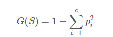
*Entropy 엔트로피 : 의사결정나무의 수학적인 개념.
엔트로피 함수는 아래와 같다.
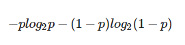

의사결정나무를 통과하기 전에는 엔트로피가 1이지만, 의사결정나무를 통과하게 되면 조건에 따라 종속변수가 종류별로 분리되므로 엔트로피는 0에 가까워진다. 엔트로피가 0에 가까울 수록 잘 분리됐다고 본다.
Information Gain : 의사결정나무의 성능 체크
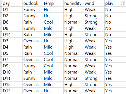
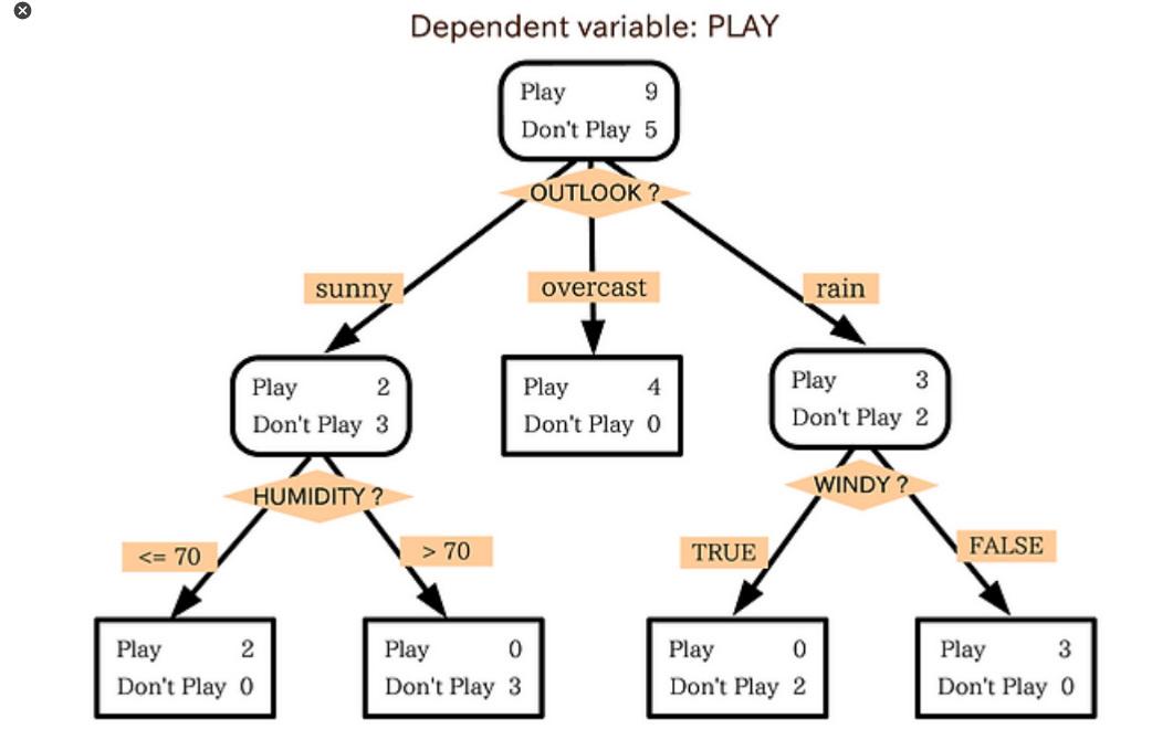
샘플 데이터가 위와 같다고 할 때, 의사결정나무를 통과하기 전의 Yes의 확률 p = 9/14 이다.
엔트로피 공식에 넣으면,

before_entropy = -(9/14) * np.log2(9/14) - (1 - (9/14)) * np.log2(1 - (9/14))
before_entropy
분기점을 통과하기 전의 엔트로피 값은 약 0.94가 나온다.
첫번째 분기점을 지나고 난 후의 확률은 각각,
Yes :4, Yes:2 NO: 3, Yes:3 No:2 으로 ,
1, 0.4, 0.6 이다.
엔트로피는 각각 계산한 후, 가중평균을 이용해서 구한다.

after_entropy_1 = 0
after_entropy_2 = -0.4 * np.log2(0.4) - (1 - 0.4) * np.log2(1 - 0.4)
after_entropy_3 = -0.6 * np.log2(0.6) - (1 - 0.6) * np.log2(1 - 0.6)
after_entropy = (4 * after_entropy_1 + 5 * after_entropy_2 + 5 * after_entropy_3) / (4 + 5 + 5)
after_entropy_1,2,3은 각각 (0, 0.9709505944546686, 0.9709505944546686)
가중평균의 엔트로피 after_entropy = 0.6935361388961919
[노드를 설정하는 방법]
- information gain이 가장 높은 변수를 root 변수로 설정
- 나머지 변수들을 information gain을 구하고 information gain이 가장 높은 변수를 다음 노드로 설정
[Iris 예제]
sklearn datasets에 내장되어있는 iris 데이터를 불러온다.
from sklearn import datasets
from sklearn.tree import DecisionTreeClassifier
iris = datasets.load_iris()

feature와 target 이 이미 나뉘어 있다.
iris data를 보기 쉽게 데이터 프레임 형태로 변환하면,
import pandas as pd
df = pd.DataFrame(iris.data, columns=iris.feature_names)

target 값들은 나오지 않는데, target 컬럼을 아래와 같이 추가한다.
df['label'] = iris.target
df.tail()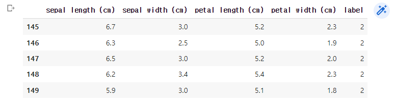
[모델의 학습]
model = DecisionTreeClassifier(max_depth=2, random_state=1).fit(iris.data, iris.target)max_depth : 몇번 분할할 것인지. 너무 많이 분할하면 overfitting 된다.
[모델 시각화]
from sklearn.tree import export_graphviz
export_graphviz(model, out_file="tree.dot", class_names = iris.target_names,
                           feature_names = iris.feature_names, impurity=True, filled=True)
import graphviz
# 위에서 생성된 tree.dot 파일을 Graphiviz 가 읽어서 시각화
with open("tree.dot") as f:
    dot_graph = f.read()
graphviz.Source(dot_graph)
※ 지니계수 : 불순도를 나타내는 지표. value = [ ] 로 주어진 데이터 분포에서의 지니계수.
[모델 평가]
Confusion Matrix
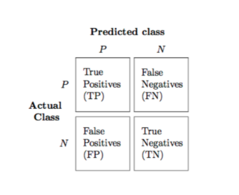
True Positives : 1인 레이블을 1이라 하는 경우를 True Positives라고 한다. -> 관심 범주를 정확하게 분류한 값.
False Negatives : 1인 레이블을 0이라 하는 경우를 False Negatives라고 한다. -> 관심 범주가 아닌것으로 잘못 분류함.
False Positives : 0인 레이블을 1이라 하는 경우를 False Positives라고 한다. -> 관심 범주라고 잘못 분류함.
True Negatives : 0인 레이블을 0이라 하는 경우를 True Negatives라고 한다. -> 관심 범주가 아닌것을 정확하게 분류.
TP/ TN 이 높고 FN/FP가 낮은게 좋음.
from sklearn.metrics import confusion_matrix
confusion_matrix(iris.target, model.predict(iris.data))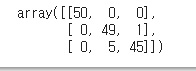
디시전트리에 의한 TP값은 49, TN은 45이다.
model.score(iris.data, iris.target)